|
Size: 21216
Comment:
|
Size: 21398
Comment:
|
| Deletions are marked like this. | Additions are marked like this. |
| Line 32: | Line 32: |
| Always check --autoclipxy for non-square images. --patchtrack=2 now works almost as good as landmark based tracking when the fiducials are not present. It should not stop you from getting to ~3Å with enough particles and good samples. It also provides a good starting point for landmark based tracking so it does not hurt to include. | Always check --autoclipxy for non-square images. --patchtrack=2 now works almost as well as landmark based tracking when the fiducials are not present. It should not stop you from getting to ~3Å with enough particles and good samples. It also provides a good starting point for landmark based tracking so it does not hurt to include it. |
| Line 43: | Line 43: |
| {{attachment:check_hand.png|Check handedness|width="600"}} Temporary files are written in tomoctf_xx if --writetmp is specified. At high tilt, i.e. tilt ID close to 0 or the number of tilt, the curve of one of the handedness (blue) should show a much deeper dip than the other one (red). If it is not obvious, something in the earlier steps might be wrong and the images might not have enough signal for CTF estimation. Also, if the dip is too close to the left or right end of the plot, consider adjusting the range of defocus search using --dfrange. |
{{attachment:check_hand.png|Check handedness|width="400"}} Temporary files are written in '''tomoctf_xx''' if `--writetmp` is specified. At high tilt, i.e. tilt ID close to 0 or the number of tilt, the curve of one of the handedness (blue) should show a much deeper dip than the other one (red). If it is not obvious, something in the earlier steps might be wrong and the images might not have enough signal for CTF estimation. Also, if the dip is too close to the left or right end of the plot, consider adjusting the range of defocus search using `--dfrange`. |
| Line 58: | Line 58: |
| Now we estimate the defocus for all tilt series. Note here we only estimate the CTF, not correct for it. The correction will happen later when extracting particles. To get to high resolution, it is often safer to use a higher than default --tilesize. | Now we estimate the defocus for all tilt series. Note here we only estimate the CTF, not correct for it. The correction will happen later when extracting particles. To get to high resolution, it is often safer to use a higher than default `--tilesize`. |
| Line 80: | Line 80: |
| Since the virus particles are quite large, here we change the reference box size to 192 using the ChangeBx button. Start from 5 positive and 5 negative references, train and apply the network, then refine the network by adding more false positives/negatives from multiple tomograms to the training set. Apply the trained network to all tomograms then close the window. Here we get 300 particles from 4 tomograms. | Since the virus particles are quite large, here we change the reference box size to 192 using the '''!ChangeBx''' button. Start from 5 positive and 5 negative references, train and apply the network, then refine the network by adding more false positives/negatives from multiple tomograms to the training set. Apply the trained network to all tomograms then close the window. Here we get 300 particles from 4 tomograms. |
| Line 87: | Line 87: |
| Extract particles of the P22 capsids. For speed and memory consumption, we use a box size of 640 and shrink the particles by 4 using --shrink. | Extract particles of the P22 capsids. For speed and memory consumption, we use a box size of 640 and shrink the particles by 4 using `--shrink`. |
| Line 96: | Line 96: |
| Since we start from the icosahedral capsid which does not have much low resolution feature, here we set --sym=icos and --res=30. Leave the rest of options as default. | Since we start from the icosahedral capsid which does not have many low resolution features, here we set `--sym=icos` and `--res=30`. Leave the rest of the options as default. |
| Line 106: | Line 106: |
| Line 114: | Line 115: |
| Now we extract particles at each penton of the capsid to refine them locally. In particle extraction, ignore the tomogram options, and only input the spt_xx/aliptcles3d_xx.lst through the --jsonali option. The program will find the particles given the refinement results. Here we want to get all 12 pentons for each capsid, so we specify --postxf=icos,0,0,35, where (0,0,35) is the coordinates of one penton from the capsid refinement. | Now we extract particles at each penton of the capsid to refine them locally. In particle extraction, ignore the tomogram options, and only input the '''spt_xx/aliptcles3d_xx.lst''' through the `--jsonali` option. The program will find the particles given the refinement results. Here we want to get all 12 pentons for each capsid, so we specify --postxf=icos,0,0,35, where (0,0,35) is the coordinates of one penton from the capsid refinement. |
| Line 122: | Line 123: |
| After extraction, instead of starting a refinement directly, gather the metadata of the newly extracted particles using the script below. The program will collect the information from particle headers so the new particles inherit the orientation and even/odd split of the previous refinement. With the --ali2d input, it also interpolate the subtilt movement of each new 2D particle from the movement of particles in the same tilt from the previous alignment. | After extraction, instead of starting a refinement directly, gather the metadata of the newly extracted particles using the script below. The program will collect the information from particle headers so the new particles inherit the orientation and even/odd split of the previous refinement. With the `--ali2d` input, it also interpolate the subtilt movement of each new 2D particle from the movement of particles in the same tilt from the previous alignment. |
| Line 128: | Line 129: |
| Now run the refinement in the same folder (spt_01) continuing from the metadata we just gathered. Here --continuefrom 0.5 will do reconstruction of iteration 1, followed by alignment of iteration 2. Since we keep the same even/odd split from the capsid refinement and particles from the two subsets still have not seen each other, we can omit the `--goldstandard` option and simply continue the refinement. | Now run the refinement in the same folder (spt_01) continuing from the metadata we just gathered. Here `--continuefrom=0.5` will do reconstruction of iteration 1, followed by alignment of iteration 2. Since we keep the same even/odd split from the capsid refinement and particles from the two subsets still have not seen each other, we can omit the `--goldstandard` option and simply continue the refinement. |
| Line 147: | Line 148: |
| This will fit B-factors based on the given map and the classical protein power spectrum, and create an 1D curve (sf.txt by default) that can be used to sharpen the structure. To visualize the results, copy the unfiltered maps to another iteration number, and rerun the last e2refine_postprocess command with the text file. | This will fit B-factors based on the given map and the classical protein power spectrum, and create a 1D curve (sf.txt by default) that can be used to sharpen the structure. To visualize the results, copy the unfiltered maps to another iteration number, and rerun the last e2refine_postprocess command with the text file. |
| Line 171: | Line 172: |
| Now get back to the capsid refinement and look for the tail of the phage with symmetry breaking. Start by making a mask covering one of the pentons along the c5 axis. It is more convenient to make the mask in Filtertool, simply using a math.linear processor to set the map to all ones, then setting the mask using mask.soft. Save the mask using File->Save, then rename it to mask_pent0.hdf | Now get back to the capsid refinement and look for the tail of the phage with symmetry breaking. Start by making a mask covering one of the pentons along the c5 axis. It is more convenient to make the mask in Filtertool, simply using a '''math.linear''' processor to set the map to all ones, then setting the mask using '''mask.soft'''. Save the mask using '''File->Save''', then rename it to '''mask_pent0.hdf'''. |
| Line 188: | Line 189: |
| In a few iterations, vague densities of the tail should show up at one side of the capsid. One easy way to visualize this is to look at the central slice views. In the e2display browser, select the map and click RngXYZ. Here we set Sum layers to 10 to look at a 20 pixel thick slice. | In a few iterations, vague densities of the tail should show up at one side of the capsid. One easy way to visualize this is to look at the central slice views. In the e2display browser, select the map and click '''RngXYZ'''. Here we set '''Sum layers''' to 10 to look at a 20 pixel thick slice. |
| Line 192: | Line 193: |
| Then we can do another run of the symmetry breaking using this as the reference, and the corresponding mask that covers the tail. Note here we do not add the --skipali option so the program will do some local alignment at the tail. To make sure the alignment does not drift too far away, we include the capsid into the mask as well. | Then we can do another run of the symmetry breaking using this as the reference, and the corresponding mask that covers the tail. Note here we do not add the `--skipali` option so the program will do some local alignment at the tail. To make sure the alignment does not drift too far away, we include the capsid into the mask as well. |
| Line 198: | Line 199: |
| There is about a 50/50 chance that the tail density appears at the top or bottom, so pick either mask_pent0.hdf or mask_pent1.hdf based on the result. After adding the capsid mask from spt_00, use threshold.clampminmax to make sure there is no value above 1 in the mask. | There is about a 50/50 chance that the tail density appears at the top or bottom, so pick either mask_pent0.hdf or mask_pent1.hdf based on the result. After adding the capsid mask from '''spt_00''', use '''threshold.clampminmax''' to make sure there is no value above 1 in the mask. {{attachment:symbreak2_msk.png|Symmetry breaking msk|width="600"}} |
| Line 222: | Line 225: |
| Then, make a mask for the tail using Filtertool, call it mask_tail1.hdf | Then, make a mask for the tail using Filtertool, call it '''mask_tail1.hdf'''. |
| Line 265: | Line 268: |
| We can still run some further classification from here, focusing on the protein-membrane interacting region and target a slightly higher resolution. | We can still run some further classification from here, focusing on the protein-membrane interacting region and targeting a slightly higher resolution. |
| Line 280: | Line 283: |
| First, expand the symmetry of the particles, and make 6 copies of each tail particle at the symmetrical orientations. `e2proclst.py` only expands the symmetry inplace so we need to make a copy of the file first. | First, expand the symmetry of the particles, and make 6 copies of each tail particle at the symmetrical orientations. `e2proclst.py` only expands the symmetry in place so we need to make a copy of the file first. |
| Line 305: | Line 308: |
| The program will compare the difference between the lst file from --ali3dold and --ali3dnew and build the eigen-trajectory from them. The 2D particle from --ali2d will define the reference frame of the movement. I.e. if you use aliptcls2d_01 instead of 03, you would see a rigid virus tail with tilting membrane. You may need to filter the 3D volume stack to visualize the features properly. Simply run | The program will compare the difference between the lst file from `--ali3dold` and `--ali3dnew` and build the eigen-trajectory from them. The 2D particle from `--ali2d` will define the reference frame of the movement. I.e. if you use aliptcls2d_01 instead of 03, you would see a rigid virus tail with a tilting membrane. You may need to filter the 3D volume stack to visualize the features properly. Simply run |
| Line 330: | Line 333: |
| One limiting factor of the visualization of high resolution features in the tomograms is the subtle local misalignment. Since we corrected for this during subtilt alignment, here we can apply those corrections back to the tomograms and improve the features inside. | One limiting factor of the visualization of high resolution features in the tomograms is the subtle local misalignment. Since we corrected this during subtilt alignment, here we can apply those corrections back to the tomograms and improve the features inside. |
Advance tutorial of EMAN2 tomography workflow
This tutorial uses a CryoET dataset of P22 bacteriophage infecting cells, which is kindly provided by Jun Liu from Yale.
The dataset contains 4 tilt series and can be downloaded here.
This tutorial contains more advanced topics, such as focused refinement and classification, symmetry breaking, and analysis of continuous motion. For new users, it is recommended to start with a simple tutorial.
Many of the functions here require an EMAN2 installation after 04/2023. A latest continuous build may work but compile from source is preferred. For the installation guide, see here.
Create project folder
Make a new empty folder for the project and 'cd' into that folder.
Make sure any EMAN2 commands you run are executed from within this folder (not any subfolder).
Import tilt series
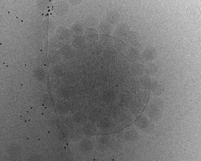
The files provided are already imported to EMAN2, so simply unzipping them in the project folder should work. For other CryoET projects, it is recommended to import the tilt series through e2projectmanager. Import tilt series will also convert them to hdf format, which greatly reduces storage (from 3.1GB to 700MB per tilt series) without obvious side effects.
Initial tomogram reconstruction
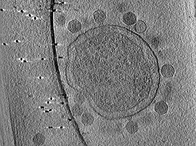
Start from one good tilt series to play with the parameters for tilt series alignment and tomogram reconstruction.
e2tomogram.py tiltseries/P22WT20210314A100.hdf --zeroid=-1 --tltstep=3.0 --npk=20 --tltkeep=0.9 --outsize=1k --niter=2,1 --bytile --pkkeep=0.9 --compressbits=8 --clipz=320 --bxsz=32 --filterres=60.0 --rmbeadthr=-1.0 --threads=12 --patchtrack=2 --autoclipxy
Always check --autoclipxy for non-square images. --patchtrack=2 now works almost as well as landmark based tracking when the fiducials are not present. It should not stop you from getting to ~3Å with enough particles and good samples. It also provides a good starting point for landmark based tracking so it does not hurt to include it.
Handedness check by CTF
e2spt_tomoctf.py tiltseries/P22WT20210314A100.hdf --dfrange=2.0,7.0,0.02 --psrange=10,15,5 --tilesize=400 --voltage=300 --cs=2.7 --nref=15 --stepx=20 --stepy=40 --checkhand --threads=1 --writetmp
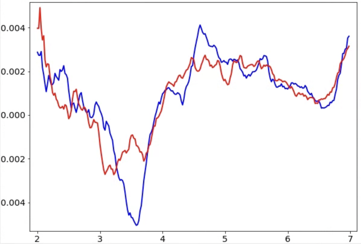
Temporary files are written in tomoctf_xx if --writetmp is specified. At high tilt, i.e. tilt ID close to 0 or the number of tilt, the curve of one of the handedness (blue) should show a much deeper dip than the other one (red). If it is not obvious, something in the earlier steps might be wrong and the images might not have enough signal for CTF estimation. Also, if the dip is too close to the left or right end of the plot, consider adjusting the range of defocus search using --dfrange.
Note this only accounts for the geometry of the tilt series, but it can still produce the wrong handedness if your individual micrographs are flipped. This can sometimes be the case with some data collection software. Even in those cases, you should still use the handedness recommended by the program (or go back and flip the raw micrographs), which will produce more stable defocus estimation.
All tomogram reconstruction
Reconstruct all tilt series using the same parameters and the tilt axis estimated by the handedness check.
e2tomogram.py --alltiltseries --zeroid=-1 --tltstep=3.0 --npk=20 --tltax=-4.2 --tltkeep=0.9 --outsize=1k --niter=2,1 --bytile --notmp --pkkeep=0.9 --compressbits=8 --clipz=320 --bxsz=32 --filterres=60.0 --moretile --rmbeadthr=-1.0 --threads=12 --patchtrack=2 --autoclipxy
CTF estimation
Now we estimate the defocus for all tilt series. Note here we only estimate the CTF, not correct for it. The correction will happen later when extracting particles. To get to high resolution, it is often safer to use a higher than default --tilesize.
e2spt_tomoctf.py --alltiltseries --dfrange=1.5,7.0,0.02 --psrange=10,15,5 --tilesize=400 --voltage=300 --cs=2.7 --nref=15 --stepx=20 --stepy=40 --threads=4
Evaluate tomograms
One convenient way to go through many tomograms in a dataset is the tomogram evaluation GUI. To use it, launch from the project manager or run
e2tomo_eval.py
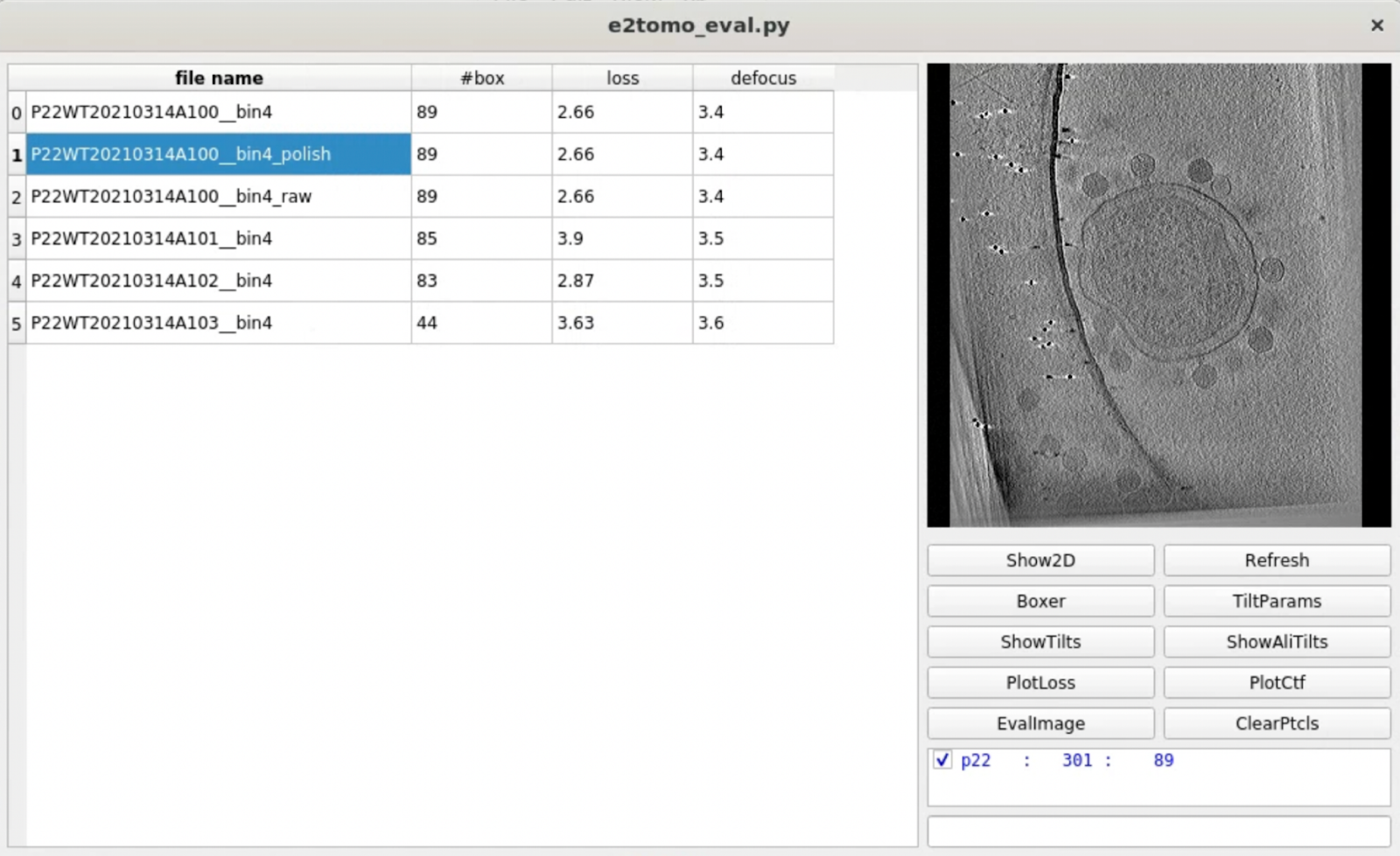
You can visualize tomograms, raw and aligned tilt series, as well as related alignment parameters from the GUI. Manual particle boxing can also be launched from the tool.
Convolutional network based particle picking
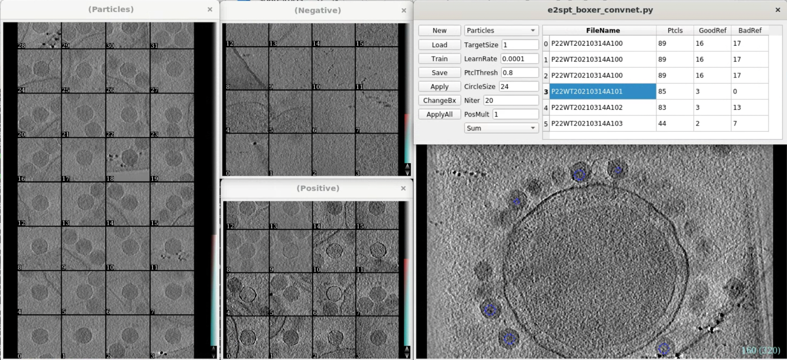
e2spt_boxer_convnet.py --label=p22
Since the virus particles are quite large, here we change the reference box size to 192 using the ChangeBx button. Start from 5 positive and 5 negative references, train and apply the network, then refine the network by adding more false positives/negatives from multiple tomograms to the training set. Apply the trained network to all tomograms then close the window. Here we get 300 particles from 4 tomograms.
Particle extraction
Extract particles of the P22 capsids. For speed and memory consumption, we use a box size of 640 and shrink the particles by 4 using --shrink.
e2spt_extract.py --boxsz_unbin=640 --label=p22 --threads=32 --alltomograms --shrink=4.0 --tltkeep=1.0 --compressbits=8 --parallel thread:8

e2spt_buildsets.py --allparticles
Initial model generation
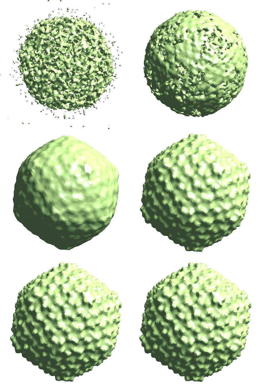
Since we start from the icosahedral capsid which does not have many low resolution features, here we set --sym=icos and --res=30. Leave the rest of the options as default.
e2spt_sgd_new.py sets/p22_bin4.lst --res=30.0 --niter=100 --shrink=1 --parallel=thread:17 --ncls=1 --batch=12 --learnrate=0.2 --sym=icos
Icosahedral capsid refinement
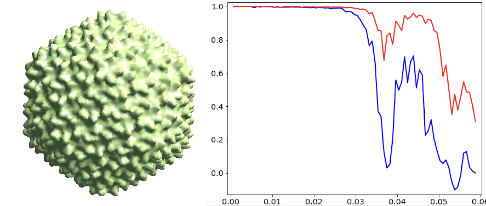
Start from the symmetrical refinement of the capsid. This should reach Nyquist of the particles (17Å) easily. One thing to note here is the FSC curve should improve after the subtilt refinement (red vs blue curve below). If it does not, it means either the data does not have enough signal per particle per tilt for the alignment, which may greatly limit the resolution achieved, or the tilt series alignment is so good that there isn’t much to improve, which does not really happen often.
e2spt_refine_new.py --ptcls=sets/p22_bin4.lst --ref=sptsgd_00/output_cls0.hdf --startres=30.0 --goldstandard --sym=icos --iters=p3,t2,p,t,r,d --keep=0.95 --parallel=thread:32 --threads=32
Penton refinement
Now we extract particles at each penton of the capsid to refine them locally. In particle extraction, ignore the tomogram options, and only input the spt_xx/aliptcles3d_xx.lst through the --jsonali option. The program will find the particles given the refinement results. Here we want to get all 12 pentons for each capsid, so we specify --postxf=icos,0,0,35, where (0,0,35) is the coordinates of one penton from the capsid refinement.
e2spt_extract.py --boxsz_unbin=190 --newlabel=capc5 --threads=32 --maxtilt=100 --padtwod=2.0 --shrink=1 --tltkeep=1.0 --jsonali=spt_00/aliptcls3d_03.lst --compressbits=8 --postxf icos,0,0,35 --mindist 100 --parallel thread:32

e2spt_buildsets.py --allparticles --label capc5
After extraction, instead of starting a refinement directly, gather the metadata of the newly extracted particles using the script below. The program will collect the information from particle headers so the new particles inherit the orientation and even/odd split of the previous refinement. With the --ali2d input, it also interpolate the subtilt movement of each new 2D particle from the movement of particles in the same tilt from the previous alignment.
e2spt_gathermeta.py --ptcls sets/capc5.lst --ali2d spt_00/aliptcls2d_04.lst
Now run the refinement in the same folder (spt_01) continuing from the metadata we just gathered. Here --continuefrom=0.5 will do reconstruction of iteration 1, followed by alignment of iteration 2. Since we keep the same even/odd split from the capsid refinement and particles from the two subsets still have not seen each other, we can omit the --goldstandard option and simply continue the refinement.
e2spt_refine_new.py --path spt_01 --continuefrom 0.5 --sym c5 --parallel thread:32 --startres 20 --tophat localwiener --localrefine --iters=p2,t2,p,t,r,d --keep=0.95 --threads=32
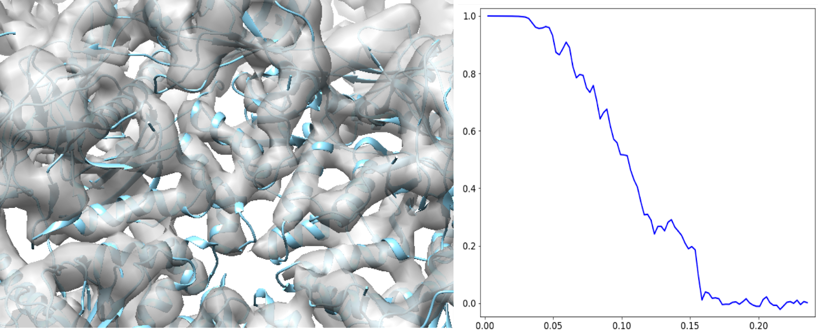
This should get better than 7Å at the end. At this point, the SSEs from the model (PDB: 5UU5) can fit in nicely.
Sharpening using structure factor
As we are achieving subnanometer resolution, it is often helpful to sharpen the map to get better real space features. Here we can run
e2spt_structfac.py --even spt_01/threed_raw_even.hdf --res 7
This will fit B-factors based on the given map and the classical protein power spectrum, and create a 1D curve (sf.txt by default) that can be used to sharpen the structure. To visualize the results, copy the unfiltered maps to another iteration number, and rerun the last e2refine_postprocess command with the text file.
cp spt_01/threed_raw_even.hdf spt_01/threed_10_even.hdf
cp spt_01/threed_raw_odd.hdf spt_01/threed_10_odd.hdf
e2refine_postprocess.py --even spt_01/threed_10_even.hdf --setsf sf.txt --tophat localwiener --threads 32 --restarget 7 --sym c5
Once created, the file can be input to other e2spt_refine_new.py runs through --setsf option to sharpen the map at every iteration.
Evaluating subtilt refinement
Run the following command to evaluate the results of a subtilt refinement.
e2spt_evalsubtlt.py --path spt_01
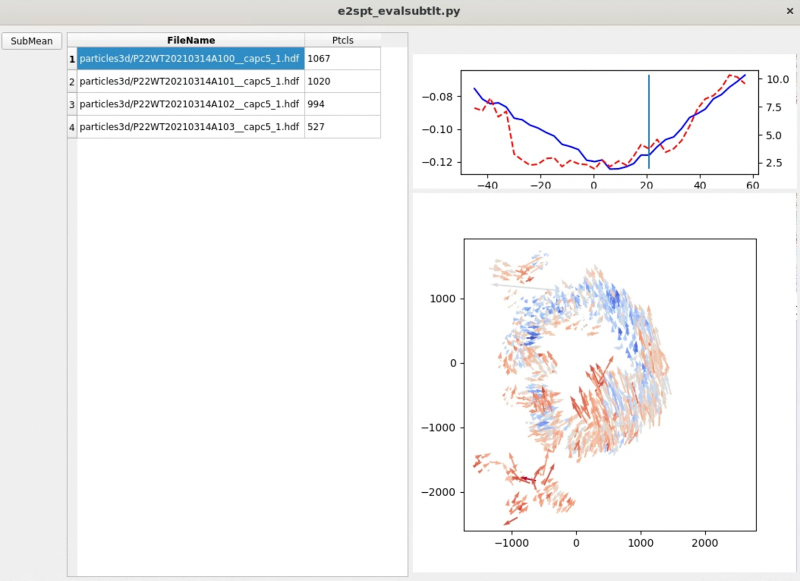
Typically, you should see the amount of movement in each tilt (red dashed line) roughly correlated with the particle score (blue line), both of which increase at higher tilt. In each tilt, the vectors should form a somewhat locally correlated flow field. Note the length of arrows are exaggerated, since they normally do not move at a length that’s visible at the scale of the entire tomogram.
Finding tail using symmetry breaking
Now get back to the capsid refinement and look for the tail of the phage with symmetry breaking. Start by making a mask covering one of the pentons along the c5 axis. It is more convenient to make the mask in Filtertool, simply using a math.linear processor to set the map to all ones, then setting the mask using mask.soft. Save the mask using File->Save, then rename it to mask_pent0.hdf.
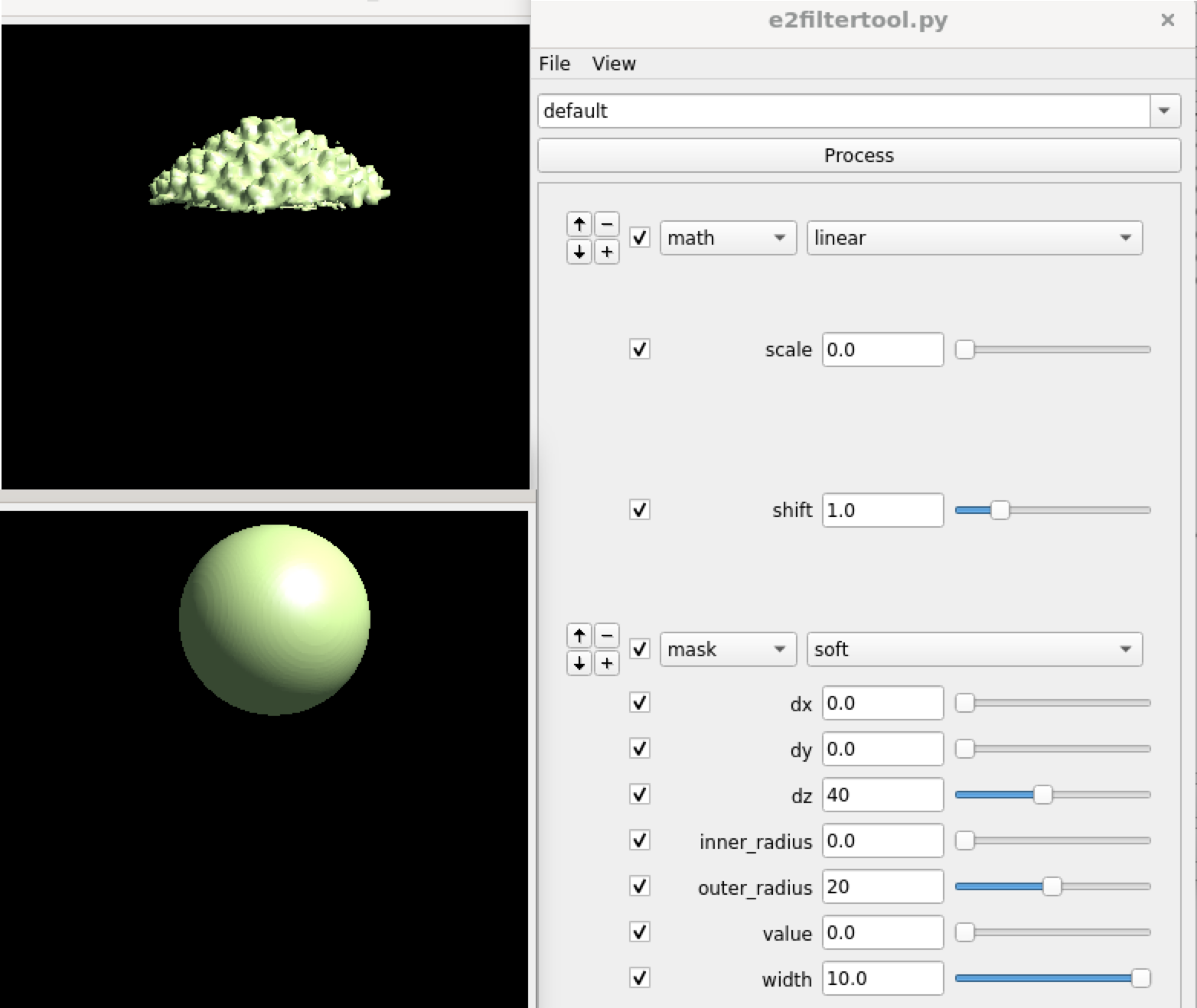
While running symmetry breaking with just this mask may work, it can be a bit tricky since the program can actually put any penton at the location of the mask without a given reference. One way to get around this is to use a mask that covers two pentons at the opposite sites, and break the icosahedral symmetry while applying the c5 symmetry, so the program will put the two pentons with the most differences at the two sites, and one of them will have the tail. So run
e2proc3d.py mask_pent0.hdf mask_pent1.hdf --rot 0,180,0
e2proc3d.py mask_pent0.hdf mask_pent2.hdf --addfile mask_pent1.hdf
Then, run
e2spt_refinemulti_new.py --nref 1 --ptcls spt_00/aliptcls3d_03.lst --niter 10 --maxres 40 --breaksym icos --loadali3d --parallel thread:32 --minres 200 --sym c5 --maskali mask_pent2.hdf --skipali
In a few iterations, vague densities of the tail should show up at one side of the capsid. One easy way to visualize this is to look at the central slice views. In the e2display browser, select the map and click RngXYZ. Here we set Sum layers to 10 to look at a 20 pixel thick slice.
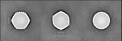
Then we can do another run of the symmetry breaking using this as the reference, and the corresponding mask that covers the tail. Note here we do not add the --skipali option so the program will do some local alignment at the tail. To make sure the alignment does not drift too far away, we include the capsid into the mask as well.
e2proc3d.py mask_pent0.hdf mask_pent0x.hdf --addfile spt_00/mask.hdf --process threshold.clampminmax:maxval=1
There is about a 50/50 chance that the tail density appears at the top or bottom, so pick either mask_pent0.hdf or mask_pent1.hdf based on the result. After adding the capsid mask from spt_00, use threshold.clampminmax to make sure there is no value above 1 in the mask.

e2spt_refinemulti_new.py sptcls_00/threed_05_00.hdf --ptcls spt_00/aliptcls3d_03.lst --niter 10 --maxres 40 --breaksym icos --loadali3d --parallel thread:32 --minres 200 --sym c5 --maskali mask_pent0x.hdf
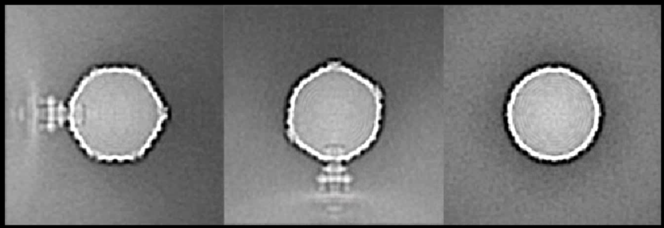
Since we are applying the c5 symmetry here, the tail will not be fully resolved, but the location of the tail should be mostly correct, which is indicated by the solid density in the structure after the refinement.
Tail refinement
Now we found the tail of each capsid, we can re-extract the particles of the base on the refinement results. To solve the structure, we still need to break the c5 symmetry of the capsid and apply the c6 symmetry of the tail.
e2spt_extract.py --boxsz_unbin=200 --newlabel=tail1 --threads=32 --maxtilt=100 --padtwod=2.0 --shrink=1 --tltkeep=1.0 --jsonali=sptcls_01/aliptcls3d_10_00.lst --compressbits=8 --postxf c1,0,0,50 --mindist 100 --parallel thread:32

e2spt_buildsets.py --allparticles --label tail1

e2spt_refinemulti_new.py --nref 1 --ptcls sets/tail1.lst --niter 10 --maxres 40 --breaksym c5 --loadali3d --parallel thread:32 --minres 200 --sym c6 --skipali
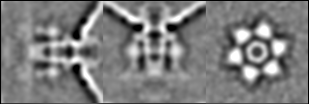
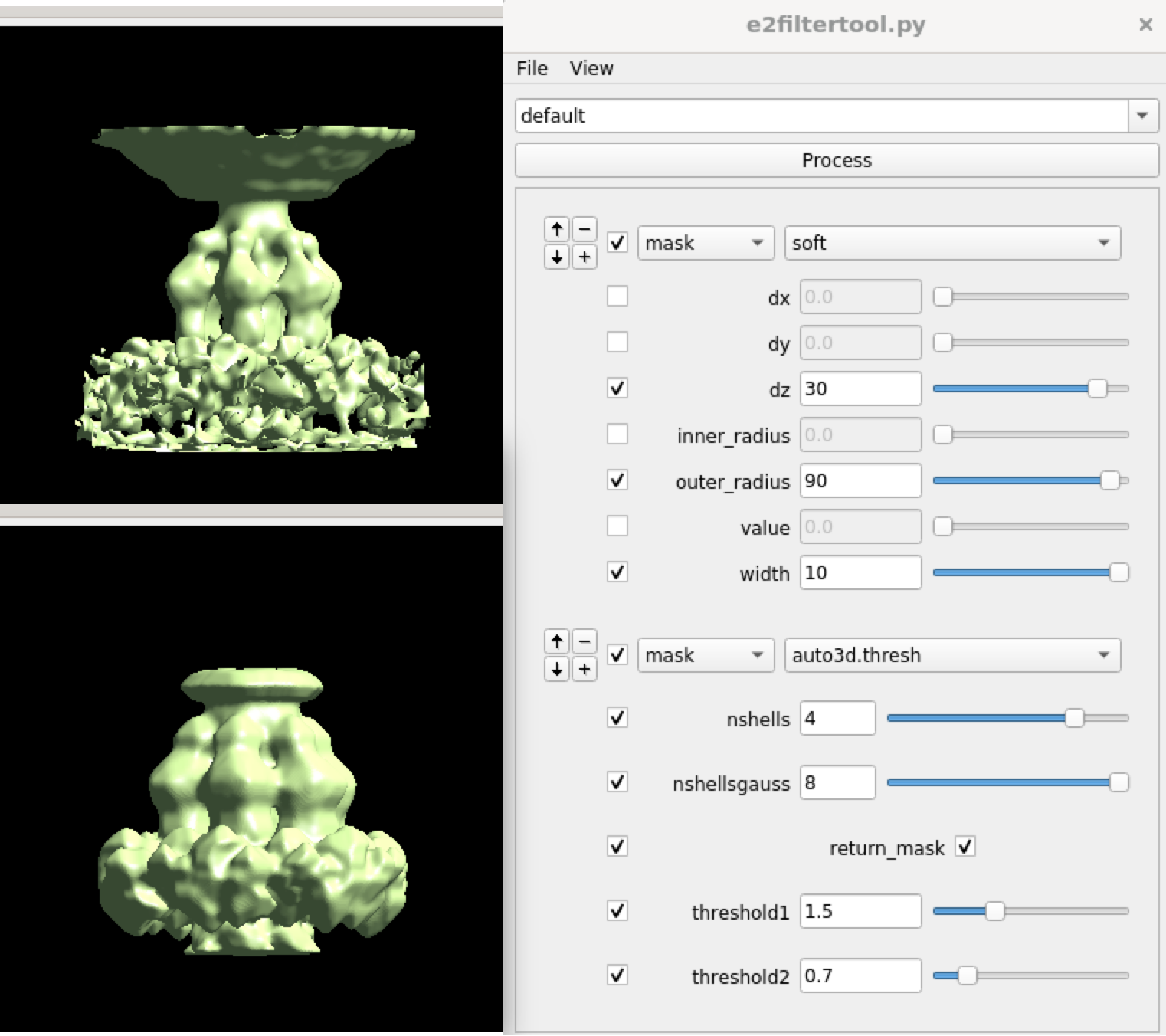
Then, make a mask for the tail using Filtertool, call it mask_tail1.hdf.
After this, we can start the refinement. First, interpolate the subtilt movement of the capsid and apply it to the nearby tail particles. Then locally refine the structure of the tail. Here we did symmetry breaking at the e2spt_refinemulti_new.py as well as e2spt_refine_new.py. It is actually okay to skip the symmetry breaking in the second refinement, but it does not hurt to do an extra round just to be safe.
e2spt_gathermeta.py --ptcls sets/tail1.lst --ali2d spt_01/aliptcls2d_07.lst --ali3d sptcls_02/aliptcls3d_10_00.lst
This creates spt_02 and compiles metadata inside. Then,
e2spt_refine_new.py --path spt_02 --continuefrom 0.5 --sym c6 --breaksym c5 --parallel thread:32 --startres 20 --tophat localwiener --localrefine --setsf sf.txt --iters=p4,t2 --keep=0.95 --threads=32 --mask mask_tail1.hdf
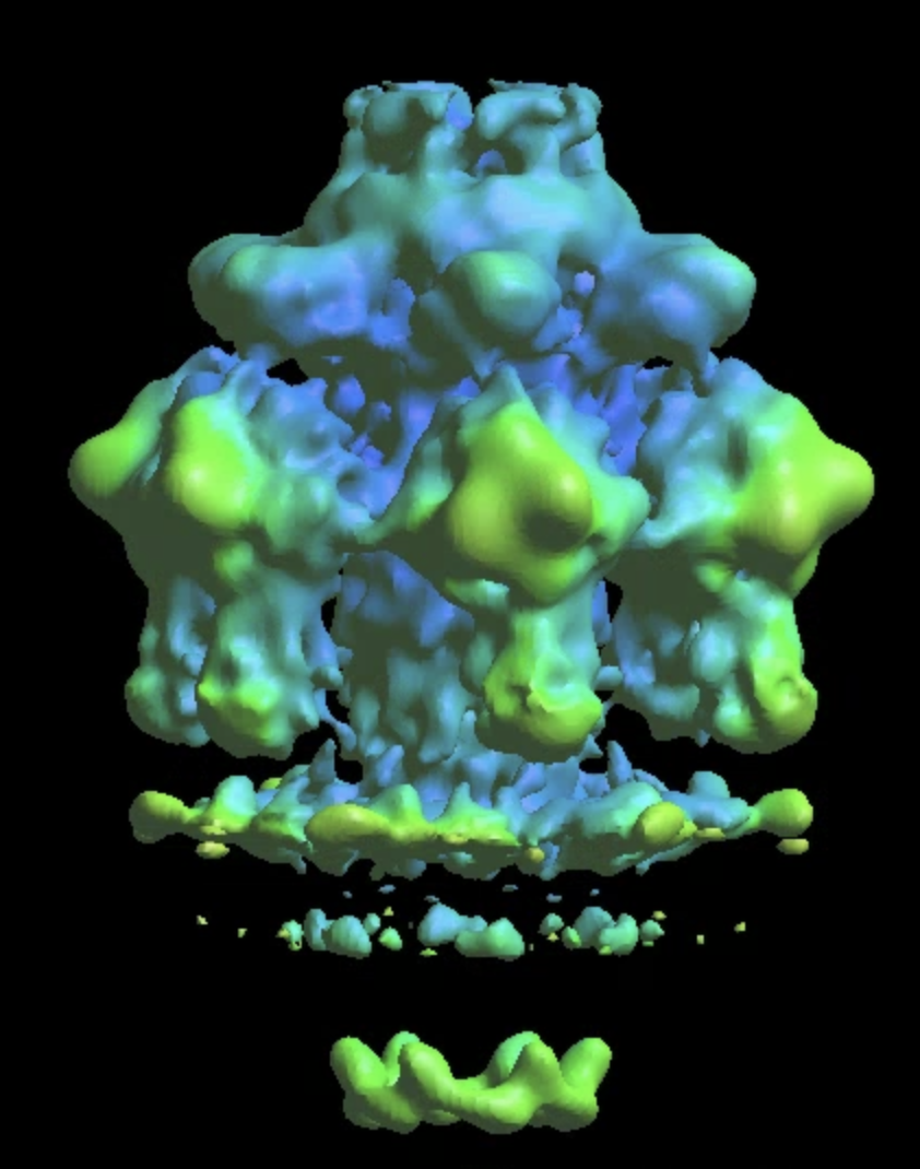
Further classification of the tail
The single model refinement will get to ~20Å resolution. One limitation of the refinement is the heterogeneity at the lower part of the tail where it interacts with the membrane. This is probably because only some of the particles are anchored on the membrane, whereas the others are floating in solution. To sort them out, do some more classification. Similarly, we create a soft mask that covers the lower part of the tail, and call it mask_tail0.hdf
e2spt_refinemulti_new.py --nref 2 --ptcls spt_02/aliptcls3d_05.lst --niter 10 --maxres 50 --loadali3d --parallel thread:32 --minres 500 --sym c6 --maskali mask_tail0.hdf --skipali
This will yield two classes, one with tails floating, and the other with tails sitting on the membrane.
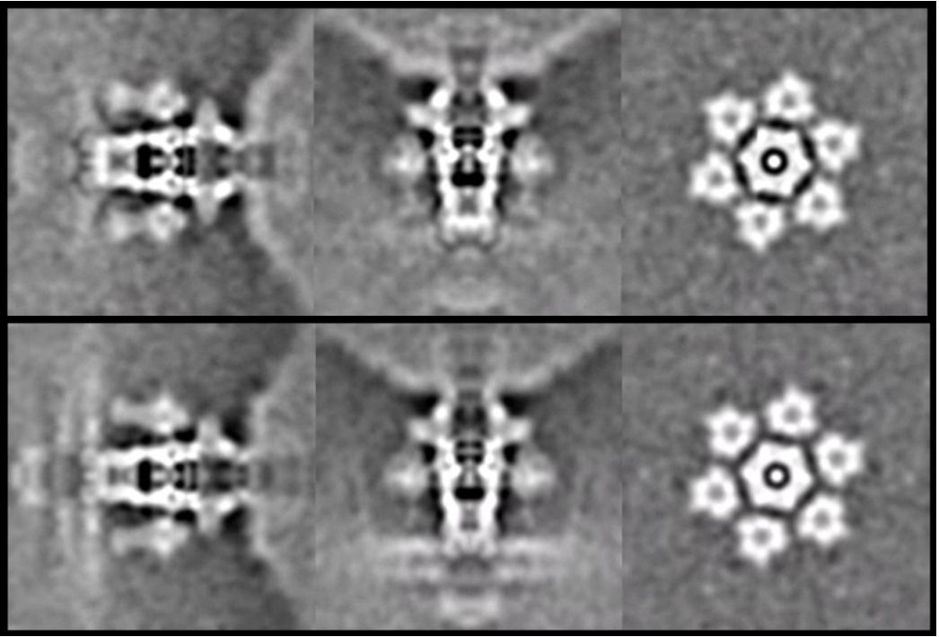
It is also possible to further refine the structure of individual classes.
e2spt_gathermeta.py --ptcls sptcls_03/aliptcls3d_10_01.lst --ali2d spt_03/aliptcls2d_07.lst --ali3d sptcls_03/aliptcls3d_10_00.lst

e2spt_refine_new.py --path spt_03 --continuefrom 0.5 --sym c1 --parallel thread:32 --startres 20 --tophat localwiener --localrefine --setsf sf.txt --iters=p4,t2,p,t,r --keep=0.95 --threads=32 --mask mask_tail1.hdf
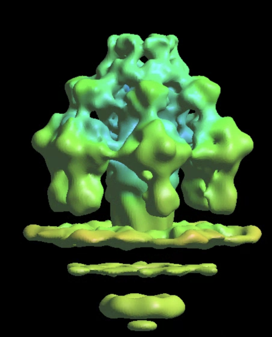
This will produce a map at ~16Å resolution, slightly better than the previous refinement despite having ~30% fewer particles. The channel through the membrane becomes more visible too.
We can still run some further classification from here, focusing on the protein-membrane interacting region and targeting a slightly higher resolution.
e2spt_refinemulti_new.py --nref 2 --ptcls spt_05/aliptcls3d_05.lst --niter 10 --maxres 30 --loadali3d --parallel thread:32 --minres 200 --sym c6 --maskali mask_tail2.hdf
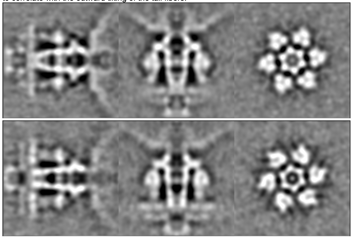
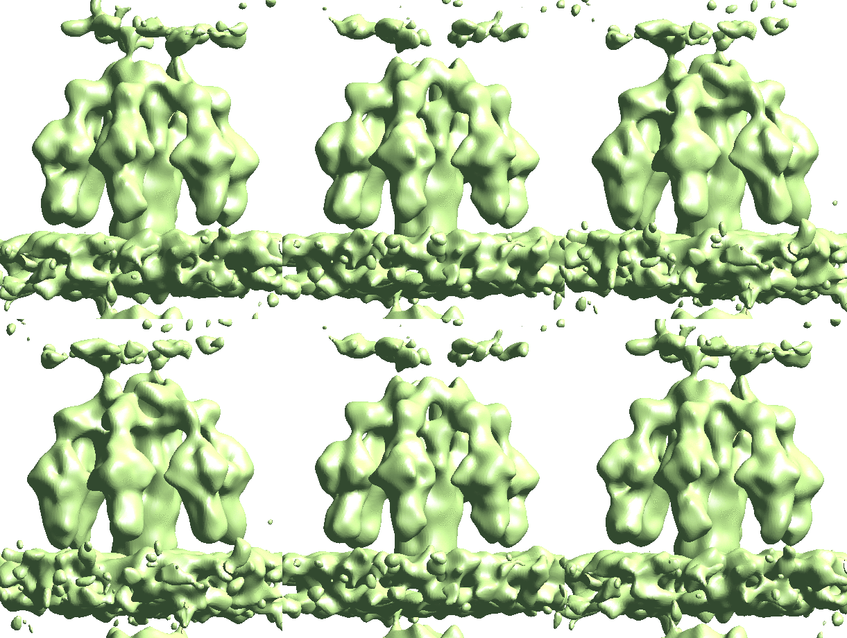
Here we can see a movement that looks like the opening and closing of the channel, which seems to correlate with the outward tilting of the tail fibers.
Continuous movement
There are probably multiple modes of continuous movement within the system, but most of them are tricky to deal with since we are very low on particle count at this moment. Here we focus on a relatively simple example, the overall tilting of the virus tail with respect to the membranes.
First, expand the symmetry of the particles, and make 6 copies of each tail particle at the symmetrical orientations. e2proclst.py only expands the symmetry in place so we need to make a copy of the file first.
cp spt_05/aliptcls3d_05.lst spt_05/aliptcls3d_05_c6.lst
e2proclst.py spt_05/aliptcls3d_05_c6.lst --sym c6
Then do a few rounds of refinement focusing on the membrane and density below.
e2spt_gathermeta.py --ptcls spt_05/aliptcls3d_05_c6.lst --ali2d spt_03/aliptcls2d_07.lst --ali3d spt_05/aliptcls3d_05_c6.lst

e2spt_refine_new.py --path spt_09 --continuefrom 0.5 --sym c1 --parallel thread:32 --startres 30 --localrefine --setsf sf.txt --iters=p3 --keep=0.95 --threads=32 --mask mask_tail5.hdf
To make sure the focused refinement works properly, take a look at the unmasked results in spt_xx/threed_raw_even/odd.hdf. Here we should see solid density of the membrane and channel, with vague densities of the virus tail above.
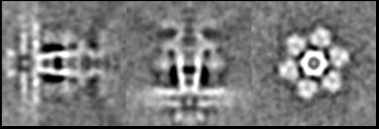
Finally, we can compile the trajectory of the continuous movement by comparing the difference of angle assignment between the two refinements.
e2spt_trajfromrefine.py --ali3dold spt_09/aliptcls3d_01.lst --ali3dnew spt_09/aliptcls3d_03.lst --maxshift 25 --nstd 3 --ali2d spt_09/aliptcls2d_03.lst --path spt_09 --nptcl 300 --nframe 8 --nbasis 1
The program will compare the difference between the lst file from --ali3dold and --ali3dnew and build the eigen-trajectory from them. The 2D particle from --ali2d will define the reference frame of the movement. I.e. if you use aliptcls2d_01 instead of 03, you would see a rigid virus tail with a tilting membrane. You may need to filter the 3D volume stack to visualize the features properly. Simply run
e2proc3d.py spt_05/threed_eig_00.hdf spt_05/threed_eig_00lp.hdf --process filter.lowpass.gauss:cutoff_freq=0.03
Then display the movie by clicking the Show All 3D button.
Map particles to tomograms
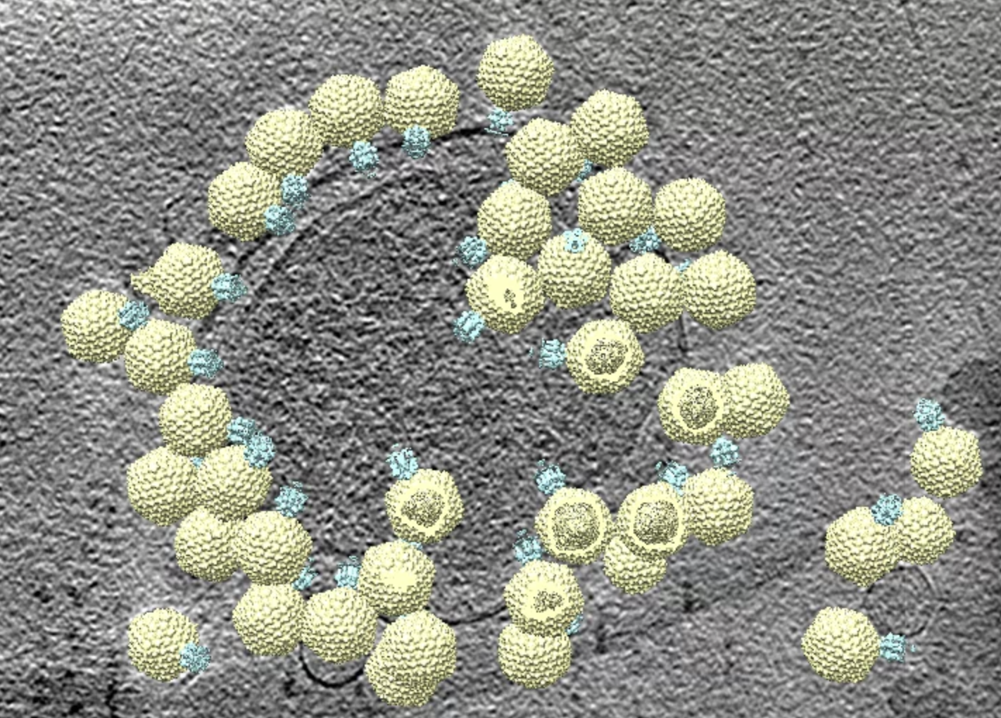
After refinement, we can map particles back to the original tomograms to visualize their organization inside the tomogram. We can also do this for multiple refinements and visualize them in the same tomogram.
e2spt_mapptclstotomo.py --new --tomo tomograms/P22WT20210314A100__bin4.hdf --path spt_00 --iter 3
e2spt_mapptclstotomo.py --new --tomo tomograms/P22WT20210314A100__bin4.hdf --path spt_03 --iter 5
e2spt_mapptclstotomo.py --new --tomo tomograms/P22WT20210314A100__bin4.hdf --path spt_04 --iter 5
Then open the raw tomogram and the mapped back particles (spt_00/ptcls_in_tomo_P22WT20210314A100_03.hdf etc.) in Chimera.
Polish tomogram using subtilt refinement
One limiting factor of the visualization of high resolution features in the tomograms is the subtle local misalignment. Since we corrected this during subtilt alignment, here we can apply those corrections back to the tomograms and improve the features inside.
e2spt_polishtomo.py --path spt_00 --fname tomograms/P22WT20210314A100__bin4.hdf --res 40
