• EMAN2
• e2tomo_more

Extra functions for EMAN2 tomography

• This page describes extra functionalities of EMAN2 tomography workflow. This tutorial is frequently updated, so it is better to have EMAN2 version as new as possible.

Generate tilt series from micrographs

If you collect tilt series using SerialEM, one simple way to import is to run motion correction for the movies, then put all output micrographs (usually mrc format) inside one folder called "micrographs" in the EMAN2 project folder. Then, run

e2buildstacks.py micrographs --tilts --guess

The program will separate the micrographs into tilt series and sort each tilt series by tilt angle, using the information from the file names. It does not always guess correctly, but works more often than not. It also deals with duplicated images. i.e., if multiple exposures are done at the same angle, only the last one will be kept. The program will compile tilt series as .lst files in the "tiltseries" folder, which can be used for the rest parts of the workflow.

Determine the handedness of a tomogram

In EMAN2 build after 05/23/2019, we can determine the handedness of a tomogram using CTF information. The idea is, at a non-zero tilt angle, one side of the specimen should be closer to the focal plane than the other one. Since this is already taken into consideration in the CTF estimation step, we just run the estimation twice on both the current and inverted hand, and check which one has a better fit.

• Find a tilt series in the dataset with good signal (at least 2 clear Thon rings). This will only work when the defocus can be determined unambiguously in the first place, so phase plate data may and may not work... Reconstruct it with tltax set empty so the program will determine the tilt angle automatically.

• Run the CTF estimation from the GUI using the correct parameters, but check the checkhand option. The program will suggest whether the hand need to be inverted at the end.

• If the hand is flipped, reconstruct the tomograms with the suggested tltax value given by the CTF estimation program. You can also run e2tomogram with --load and --flip with 0 iterations to skip the alignment.

• Note this only accounts for the geometry of the tilt series, but it can still produce the wrong handedness if your individual micrographs are flipped. This can sometimes be the case with some data collection software. Even in those cases, you should still use the handedness recommended by the program (and flip the raw micrographs), which will produce more stable defocus estimation.

Automated particle selection

A new tool (post 2.91) is implemented for CNN guided automated particle selection from tomograms. The concept is similar to the tomogram segmentation protocol, but a number of changes have been made to improve the accuracy and throughput of the process. A new GUI has been made to simplify the training process. Note that this requires a CUDA compatible GPU and tensorflow setup to work. To use see Subtomogram Averaging -> Convnet based auto-boxing or manually run

•  e2spt_boxer_convnet.py --label xxx

Here label will be the label of the newly selected particle. This will bring up three windows: the main window with various options and a list of tomograms, and two windows (should be empty in the beginning) for positive and negative samples. Clicking any tomogram in the list will bring up two other windows: the slice view of the tomogram and the list of particles under the given label. Here is a simple workflow.

1. Select a few (>5) positive to negative samples. On the tomogram slice view, left-click to select positive samples, and Ctrl+left-click to select negative samples. Shift-click an image in the sample list to delete it. The particles should be well-centered in the positive samples, and there should not be particles in the center of negative samples.

2. Click Train to start training and some output will be printed in the command line. Keep clicking Train (or use a larger Niter) until the loss stops decreasing (or whenever you want to stop).

3. Click Apply to let the program select particles using the trained network.

4. Go through the particle list, Ctrl+left-click a falsely recognized particle to add it to the list of negative samples (left-click a particle will add it to the positive samples, but it is not very necessary since they are selected by the network already). You can also go through the tomogram again to add a few particles that are not selected by the network into the positive samples.

5. Click Train again to re-train the network using the new training set, and click Apply to inspect its results.

6. Repeat the process until the neural network's performance is satisfying. You can also select other tomograms in the list, to test the performance of the model and add more positive/negative samples to the training set.

7. Go through all tomograms in the list and apply the network to select the particles. These particles can be viewed and modified in e2spt_boxer.py, and extracted through the particle extraction steps of the main workflow.

   

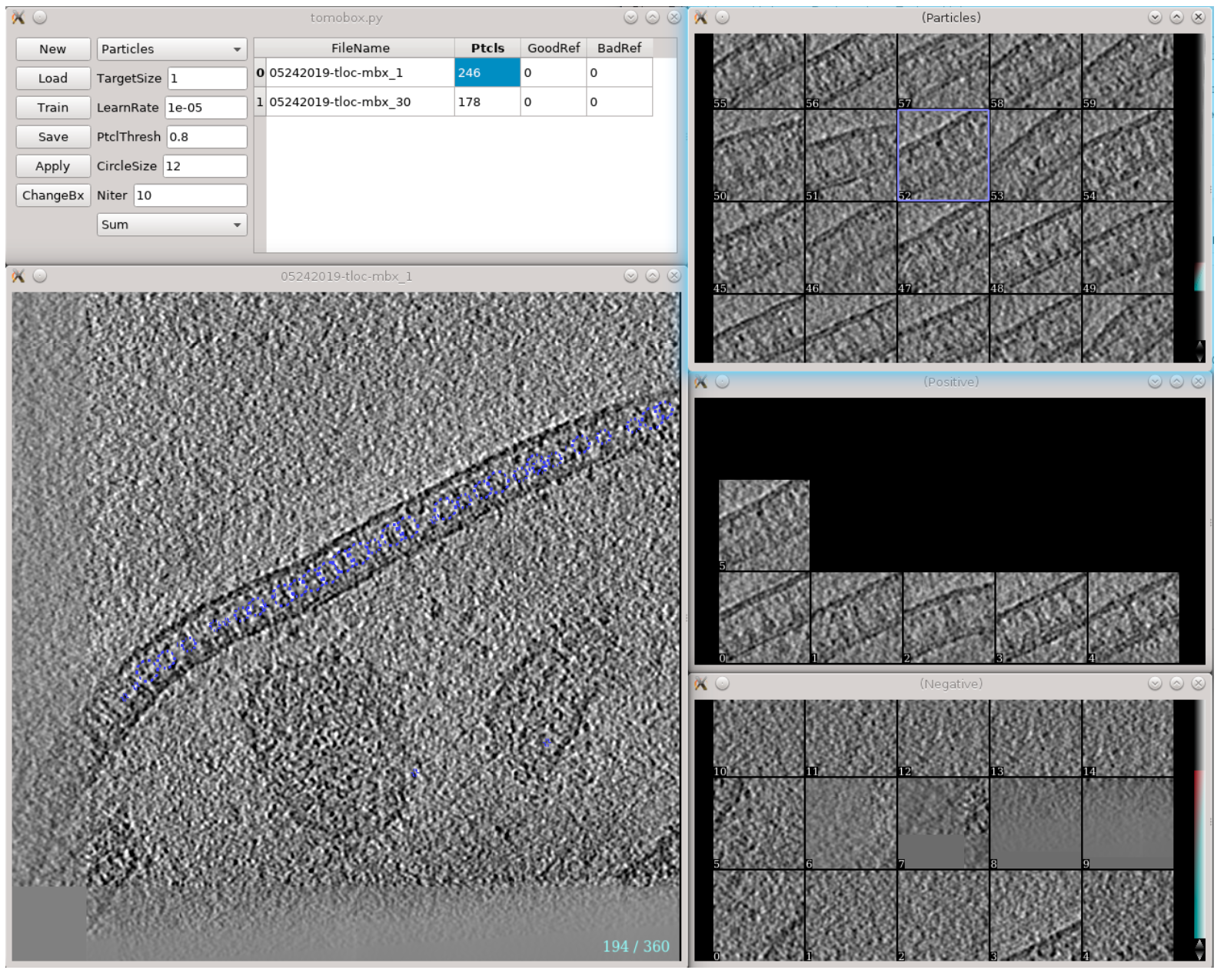
Description of items on the GUI:

• New/Save/Load: Initialize a new CNN / save the current trained network to disk / load a trained network from disk.

• ChangeBx : Change the box size of positive/negative samples. Ideally, the particles should be recognizable visually from the reference images. The process can be slow if the references come from multiple tomograms.

• Reference/Particle selection box: Display circles of references or particles in the tomogram slice view.

• TargetSize : This controls the size of target area used for CNN training. i.e. particles should be centered in this region in positive samples, and there should not be particle features in this region in negative samples. The region is defined as a Gaussian function and value here is the sigma of the Gaussian.

• Learnrate : Learning rate for the CNN training. Normally no need to change this...

• PtclThresh : The intensity threshold in the neural network output to be recognized as a particle. The target of positive samples should be 1 and negative samples should be 0.

• CircleSize : The radius of circles in pixels on the tomogram slice view. This also controls the closest distance between particles.

• Sum/Max selection box : Choose between different modes of the loss function. Sum is used for globular particles that are generally confined in the target area. In Max mode, the CNN only assume there are particle features that exist within the region. It is harder to train than the Sum mode, but allows particles of irregular shapes, such as protein fibers.

Visualize particles in tomograms

There is a simple tool to map the averaged structure to the determined position and orientation of each particle in a tomogram. Available after EMAN2.3. In versions after 05/23/2019, the function is moved to the Analysis and Visualization section in the GUI.

• Subtomogram Averaging -> Map particles to tomograms

  • Set path to be one of the spt_XX folder (not the subtlt ones).

  • Set iter to be the iteration you want to use from the refinement.

  • Browse for one tomogram you want to map the particles to.
  • If you used the new e2spt_refine_new program for the refinement:

    • you will also need to add the --new option. If this isn't shown in the GUI, go to the Command tab and add it to the end of the command before Launch

    • the program will only work with 'p' iterations, where 3-D alignment parameters are determined.

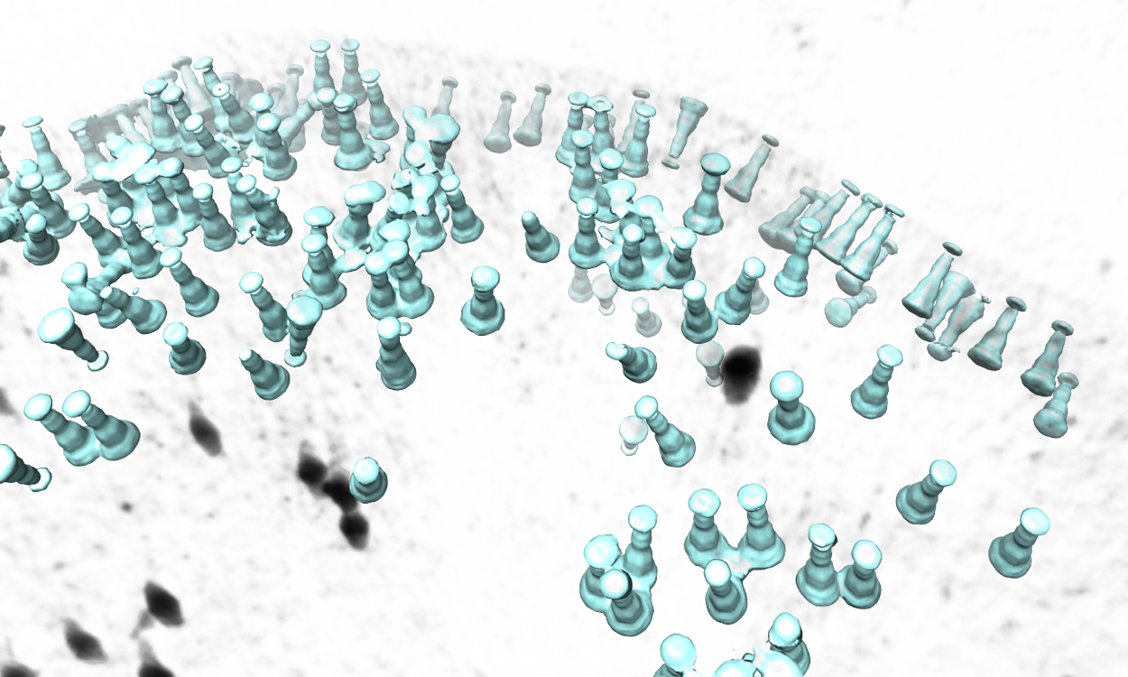
The program will then find all particles in the selected tomogram that are used in the refinement, map the averaged structure back, and produce a file called ptcls_in_tomo_xx_yy.hdf, where xx is the name of tomogram and yy is the number of iteration used. This is sometimes quite useful for objects in a cellular environment (when membrane proteins are obviously upside down for example). Image rendered with Chimera.

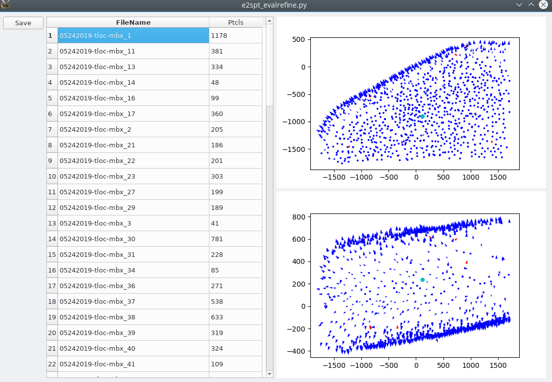
In versions after 07/09/2020, there is a simpler tool to visualize particles in tomograms. The script is called e2spt_evalrefine.py, but at present it only works with results from the older refinement pipeline. Run

e2spt_evalrefine_gui.py spt_xx/particle_parms_xx.json --mode rad

to visualize particle orientations in both x-y and x-z plane. Note that the particles need to be aligned to the symmetry axis for this to be useful. You can also click a point in the plot and the program will mark particles that point to orientation opposite to the direction from the point to the particle. Click save and the program will save another json file with the orientation of those particles inverted. There is another mode called line, that invert particle orientation based on a global vector, which can be useful for in situ protein filament arrays.

Filament refinement

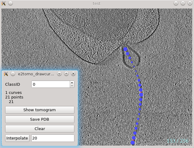
A specialized GUI is implemented for the selection of filament particles in 2.31 or later versions. In the Evaluate Tomograms window, select a tomogram, hold Shift and click the Boxer button. You can also find this through Segmentation -> Manual segmentation -> Draw curve. This will bring up a 2D tomogram viewing window and a small control panel. The following tomogram is from Caltech ETDB.

In the tomogram window, press up or down arrow (`/1 also works)to go through the slices. Use left-click to add a point on the filament, and Shift-click to delete a point. The program will build a curve that goes through all the points while minimizing the total length in 3D, so the order of adding points on the curve is irrelevant. One can select the two ends of filament and then adding points in the middle to adjust the curvature. Ctrl-click to add a point on a new curve or select an existing curve.

On the control panel, the Interpolate button will interpolate the points on all curves with a constant spacing. This will only change the visual appearance in the GUI, as well as the particle count from the Evaluate tomogram window, but the number of actual 3D particle extracted from the tomograms is controlled later in the particle extraction step. The Save PDB button will save the curves as a PDB file, so they can be visualized together with the tomograms in Chimera. Due to the limitation of PDB format, the curves are saved in pixel units, so you will need to change the voxel size of the corresponding tomogram to 1 so they overlap with the model.

When multiple types of filaments exist in the same dataset, they should be labeled separately. Use the small text box at the top of the control panel to switch between different types of filaments. The filament particles can be viewed from the Evaluate Tomograms window as curve_00, curve_01 etc. Make sure the indices of the curves are consistent throughout the dataset (i.e. when a type of filament is labeled as 01 in one tomogram, it should always be 01 even if the type 00 filament does not exist in a tomogram). After selecting the curves, to extract a certain type of filament particles from the tomogram, in the Extract particles step, set curves be the index of the filament class, and curves_overlap to be the overlap between neighboring boxes (so the spacing between boxes is box size related). It is also recommended to name the extracted particles using the newlabel option.

If the 3D particles are extracted based on the curve boxing tool, their directions along the curve are saved in the header which can be used by downstream alignment. In the initial model generation (e2spt_sgd_new.py), a command-line only option --curve will build an initial model while keeping the filament orientation of the particles. The same option is also present in subtomogram refinement (e2spt_refine_new.py) that constrains the orientation search around the filament direction.

Filling missing wedge in tomograms

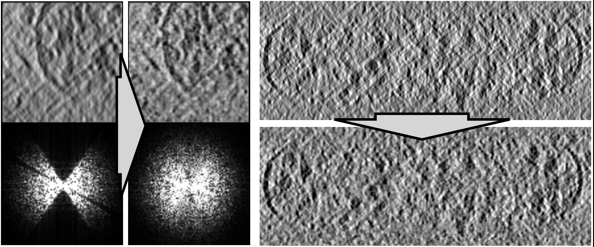
In EMAN2 build after 03/20/2020, there is a new deep learning based tool to fill in the missing wedge in raw tomograms with somewhat meaningful information. The idea is similar to a "style transform" that makes the features in the x-z 2D slice views similar to the x-y slice views. To use, run

• e2tomo_mwfill.py --train tomograms/xxx__bin4.hdf --apply tomograms/xxx__bin4.hdf,tmograms/yyy__bin4.hdf

There is no human input needed as the program will build training sets by itself. You can train and apply to the same tomogram to improve performance, or load a trained network and apply to many tomograms to save time. Note that the missing wedge filling here happens locally (you can specify box size in the program, but the performance may decrease as the box size gets larger), so it does not deal with large scale effect like the artifacts from a high contrast object, or the entire piece of invisible flat membrane.

Here is a before/after comparison of the x-z slice view of a cellular tomogram (EMPIAR-10499).

Structure factor based map sharpening

Many programs through the subtomogram refinement pipeline takes a structure factor file that is used to sharpen the density map. Unlike the single particle analysis, here we cannot generate a structure factor at the CTF estimation step since it is done in a per micrograph level. There are a few ways to generate a structure factor file for sharpening. If there is a high resolution structure of a similar protein, simply run

e2proc3d.hdf emd.hdf emd.hdf --calcsf structfac.txt

Alternatively, if you get an unsharpened structure from subtomogram averaging already, a structure factor file can be computed from it using

e2spt_structfac.py threed_xx.hdf --sfout structfac.txt

The program will fit two B-factors to the given density map, so the Fourier space intensity falloff at high resolution (<20A by default) is as close to the ideal protein power spectrum as possible. This is best done using unmasked average structures. So instead of give it a single threed_xx.hdf map, it is sometimes more convienient to provide the even file and the program will look for the corresponding odd map.

e2spt_structfac.py --even spt_xx/threed_raw_even.hdf --sfout structfac.txt

If CTF correction is performed previously, you can also include the label of the particles (the string used in particle picking and extraction) so the program will correct for the low resolution amplitude artifact of the averaged structure using the CTF information. Simply run

e2spt_structfac.py --even spt_xx/threed_raw_even.hdf --sfout structfac.txt --label xxx

Once a structure factor file is generated, it can be provided to various EMAN2 programs using the --setsf option, and the sharpending will be performed automatically.

Note that the structure factor will be different for different proteins, so you will need to keep separate files if multiple proteins are studied from the same datasets.